Deep double descent explained (¾)

15/06/2021

The role of inductive biases with two linear examples (linear regression with gaussian noise & Random Fourier Features)

This series of blog posts was co-written with Marc Lafon. Pdf version is available here as well.

\[ \global\def\norm#1{\lVert #1 \rVert} \global\def\1{\mathbb{I}} \global\def\N{\mathcal{N}} \global\def\R{\mathbb{R}} \global\def\E{\mathbb{E}} \global\def\argmin{\text{argmin}} \global\def\Ap{A_{\sim p}} \global\def\Aq{A_{\sim q}} \global\def\Xp{X_{\sim p}} \global\def\Xq{X_{\sim q}} \global\def\p#1{#1_{\sim p}} \global\def\q#1{#1_{\sim q}} \global\def\vp{v_{\sim p}} \global\def\vq{v_{\sim q}} \global\def\xp{x_{\sim p}} \global\def\xq{x_{\sim q}} \global\def\yp{y_{\sim p}} \global\def\yq{y_{\sim q}} \global\def\wp{w_{\sim p}} \global\def\wq{w_{\sim q}} \]

In this post, we consider two settings where double descent can be empirically observed and mathematically justified, in order to give the reader some intuition on the role of inductive biases. The next post concludes with some references to recent related works studying optimization in the over-parameterized regime, or linking the double descent to a physical phenomenon named jamming.

Fully understanding the mechanisms behind this phenomenon in deep learning remains an open question, but inductive biases (introduced in the previous post) seem to play a key role.

In the over-parameterized regime, empirical risk minimizers are able to interpolate the data. Intuitively :

• Near the interpolation point, there are very few solutions that fit the training data perfectly. Hence, any noise in the data or model mis-specification will destroy the global structure of the model, leading to an irregular solution that generalizes badly (figure with \(d=20\)).
• As effective model capacity grows, many more interpolating solutions exist, including some that generalize better and can be selected thanks to the right inductive bias, e.g. smaller norm (figure with \(d=1000\)), or ensemble methods.

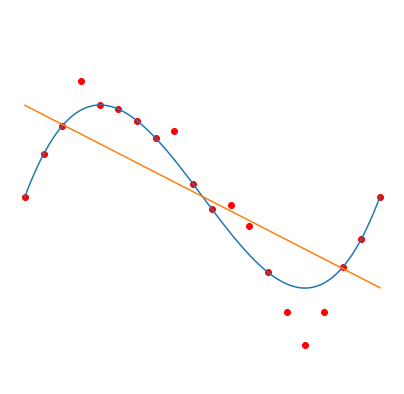
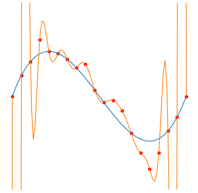
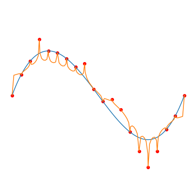
Fitting degree \(d\) Legendre polynomials (orange curve) to \(n=20\) noisy samples (red dots), from a polynomial of degree 3 (blue curve). Gradient descent is used to minimize the squared error, which leads to the smallest norm solution (considering the norm of the vector of coefficients). Taken from this blog post.

Left: \(d=1\), middle: \(d=20\), right: \(d=1000\)

Linear Regression with Gaussian Noise

In this section we consider the family class \((\mathcal{H}_p)_{p\in\left[ 1,d\right]}\) of linear functions \(h:\R^d\mapsto \R\) where exactly \(p\) components are non-zero (\(1\leq p\leq d\)). We will study the generalization error obtained with ERM when increasing \(p\) (which is regarded as the class complexity).

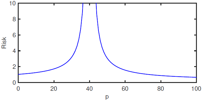
Plot of risk \(\E[(y-x^T\hat{w})^2]\) as a function of \(p\), under the random selection model of the subset of \(p\) features. Here \(\norm{w}^2=1\), \(\sigma^2=1/25\), \(d=100\) and \(n=40\). Taken from Belkin et al., 2020 ¹.

The class of predictors \(\mathcal{H}_p\) is defined as follow:

Definition 17. For \(p \in \left[ 1,d\right]\), \(\mathcal{H}_p\) is the set of functions \(h:\R^d\mapsto \R\) of the form:

\[ h(u)=u^Tw,\quad \text{for }u \in \R^d \]

With \(w \in \R^d\) having exactly \(p\) non-zero elements.

Let \((X, \mathbf{\epsilon})\in \R^d\times\R\) be independent random variables with \(X \sim \N(0,I)\) and \(\mathbf{\epsilon} \sim \N(0,\sigma^2)\). Let \(h^* \in \mathcal{H}_d\) and define the random variable

\[Y=h^*(X)+\sigma \mathbf{\epsilon}=X^Tw+\sigma \mathbf{\epsilon}\]

with \(\sigma>0\) with \(w \in \R^d\) defined by \(h^*\). We consider \((X_i, Y_i)_{i=1}^n\) \(n\) iid copies of \((X,Y)\). We are interested in the following problem:

\[ \min_{h\in \mathcal{H}_d}\E[(h(X) - Y)^2] \tag{5} \]

Let \(\mathbf{X}\in \R^{n\times d}\) the random matrix which rows are the \(X_i^T\) and \(\mathbf{Y} =(Y_1,.., Y_n)^T \in \R^n\). In the following we will assume that \(\mathbf{X}\) is full row rank and that \(n \ll d\). Applying empirical risk minimization we can write:

\[ \min_{z\in \R^d} \frac{1}{2}\norm{\mathbf{X} z - \mathbf{Y}}^2 \tag{6} \]

Definition 18 (Random p-submatrix/p-subvector) The notation used for the random p-submatrix and random p-subvector is not common and is introduced for clarity.. For any \((p,q) \in \left[ 1, d\right]^2\) such that \(p+q=d\) and matrix \(\mathbf{A} \in \R^{n\times d}\) and column vector \(v\in \R^d\), we will denote by \(\mathbf{\Ap}\) (resp. \(\vp\)) the sub-matrix (resp. sub-vector) obtained by randomly selecting a subset of p columns (resp. elements), and by \(\mathbf{\Aq} \in \R^{n\times q}\) and \(\vq\in \R^{q}\) their discarded counterpart.

In order to solve (6) we will search for a solution in \(\mathcal{H}_p \subset \mathcal{H}_d\) and increase \(p\) progressively which is a form of structural empirical risk minimization as \(\mathcal{H}_p \subset \mathcal{H}_{p+1}\) for any \(p<d\).

Let \(p \in \left[ 1, d\right]\), we are then interested in the following sub-problem:

\[ \min_{z\in \R^p} \frac{1}{2}\norm{\mathbf{\Xp} z - \yp}^2 \]

We have seen in proposition 12 of the previous post that the least norm solution is \(\p{\hat w}=\mathbf{\Xp}^+\yp\). If we define \(\q{\hat w} := 0\) then we will consider as a solution of the global problem (5) \(\hat w:=\phi_p(\p{\hat w},\q{\hat w})\) where \(\phi_p: \R^p\times\R^{q}\mapsto \R^d\) is a map rearranging the terms of \(\p{\hat w}\) and \(\q{\hat w}\) to match the initial indices of \(w\).

Theorem 19. Let \((x, \epsilon)\in \R^d\times\R\) independent random variables with \(x \sim \N(0,I)\) and \(\epsilon \sim \N(0,\sigma^2)\), and \(w \in \R^d\). we assume that the response variable \(y\) is defined as \(y=x^Tw +\sigma \epsilon\). Let \((p,q) \in \left[ 1, d\right]^2\) such that \(p+q=d\), \(\mathbf{\Xp}\) the randomly selected \(p\) columns sub-matrix of X. Defining \(\hat w:=\phi_p(\p{\hat w},\q{\hat w})\) with \(\p{\hat w}=\mathbf{\Xp}^+\yp\) and \(\q{\hat w} = 0\).

The risk of the predictor associated to \(\hat w\) is:

\[ \E[(y-x^T\hat w)^2] = \begin{cases} (\norm{\wq}^2+\sigma^2)(1+\frac{p}{n-p-1}) &\quad\text{if } p\leq n-2\\ +\infty &\quad\text{if }n-1 \leq p\leq n+1\\ \norm{\wp}^2(1-\frac{n}{p}) + (\norm{\wq}^2+\sigma^2)(1+\frac{n}{p-n-1}) &\quad\text{if }p\geq n+2\end{cases} \]

Proof. Because \(x\) is zero mean and identity covariance matrix, and because \(x\) and \(\epsilon\) are independent:

\[ \begin{aligned} \E\left[(y-x^T\hat w)^2\right] &= \E\left[(x^T(w-\hat w) + \sigma \epsilon)^2\right] \\ &= \sigma^2 + \E\left[\norm{w-\hat w}^2\right] \\ &= \sigma^2 + \E\left[\norm{\wp-\p{\hat w}}^2\right]+\E\left[\norm{\wq-\q{\hat w}}^2\right] \end{aligned} \]

and because \(\q{\hat w}=0\), we have:

\[ \E\left[(y-x^T\hat w)^2\right] = \sigma^2 + \E\left[\norm{\wp-\p{\hat w}}^2\right]+\norm{\wq}^2 \]

The classical regime (\(p\leq n\)) as been treated in Breiman & Freedman, 1983 ². We will then consider the interpolating regime (\(p \geq n\)). Recall that X is assumed to be of rank \(n\). Let \(\eta = y - \mathbf{\Xp} \wp\). We can write :

\[ \begin{aligned} \wp-\p{\hat w} &= \wp - \mathbf{\Xp}^+y \\ &= \wp - \mathbf{\Xp}^+(\eta + \mathbf{\Xp} \wp) \\ &= (\mathbf{I}- \mathbf{\Xp}^+\mathbf{\Xp})\wp - \mathbf{\Xp}^+ \eta \end{aligned} \]

It is easy to show (left as an exercise) that \((\mathbf{I}- \mathbf{\Xp}^+\mathbf{\Xp})\) is the matrix of the orthogonal projection on \(\text{Ker}(\mathbf{\Xp})\). Furthermore, \(-\mathbf{\Xp}^+ \eta \in \text{Im}(\mathbf{\Xp}^+)=\text{Im}(\mathbf{\Xp}^T)\). Then \((\mathbf{I}- \mathbf{\Xp}^+\mathbf{\Xp})\wp\) and \(-\mathbf{\Xp}^+ \eta\) are orthogonal and the Pythagorean theorem gives:

\[ \norm{\wp-\p{\hat w}}^2 = \norm{(\mathbf{I}- \mathbf{\Xp}^+\mathbf{\Xp})\wp}^2 + \norm{\mathbf{\Xp}^+ \eta}^2 \]

We will treat each term of the right hand side of this equality separately.

• \(\norm{(\mathbf{I}- \mathbf{\Xp}^+\mathbf{\Xp})\wp}^2\)

  \(\mathbf{\Xp}^+\mathbf{\Xp}\) is the matrix of the orthogonal projection on \(\text{Im}(\mathbf{\Xp}^T)=\text{Im}(\mathbf{\Xp}^+)\), then using again the Pythagorean theorem gives:

  \[ \norm{(\mathbf{I}- \mathbf{\Xp}^+\mathbf{\Xp})\wp}^2 = \norm{\wp}^2 - \norm{\mathbf{\Xp}^+\mathbf{\Xp}\wp}^2 \]

  Because \(\mathbf{\Xp}^+\mathbf{\Xp}\) is the matrix of the orthogonal projection on \(\text{Im}(\mathbf{\Xp}^T)\) we can write \(\mathbf{\Xp}^+\mathbf{\Xp}\wp\) as a linear combination of rows of \(X_p\), then using the fact that the \(x_i\) are i.i.d and of standard normal distribution we have:

  \[ \E[\norm{\mathbf{\Xp}^+\mathbf{\Xp}\wp}^2] = \norm{\wp}^2\frac{n}{p}\quad \]

  then

  \[ \E[\norm{(\mathbf{I}- \mathbf{\Xp}^+\mathbf{\Xp})\wp}^2] = \norm{\wp}^2(1-\frac{n}{p}) \]

• \(\norm{\mathbf{\Xp}^+ \eta}^2\):

  The calculation of this term used the “trace trick” and the notion of distribution of inverse-Wishart for pseudo-inverse matrices and is beyond the scope of this lecture. It can be shown that:

  \[ \E[\norm{\mathbf{\Xp}^+ \eta}^2]= \begin{cases} (\norm{\wq}^2+\sigma^2)(\frac{n}{p-n-1}) &\quad\text{if } p\geq n+2\\ +\infty &\quad\text{if }p \in \{n,n+1\} \end{cases} \]

◻

Corollary 1. Let \(T\) be a uniformly random subset of \(\left[ 1, d\right]\) of cardinality p. Under the setting of Theorem 19 and taking the expectation with respect to \(T\), the risk of the predictor associated to \(\hat w\) is:

\[ \E[(Y-X^T\hat w)^2] = \begin{cases} \left((1-\frac{p}{d})\norm{w}^2+\sigma^2\right)(1+\frac{p}{n-p-1}) &\quad\text{if } p\leq n-2\\ \norm{w}^2\left(1-\frac{n}{d}(2- \frac{d-n-1}{p-n-1})\right) +\sigma^2(1+\frac{n}{p-n-1}) &\quad\text{if }p\geq n+2\end{cases} \]

Proof. Since T is a uniformly random subset of \(\left[ 1, d\right]\) of cardinality p:

\[ \E[\norm{\wp}^2] = \E[\sum_{i\in T}w_i^2]= \E[\sum_{i=1}^{d}w_i^2 \1_{T}(i) ]=\sum_{i=1}^{d}w_i^2 \E[\1_{T}(i) ]=\sum_{i=1}^{d}w_i^2 > \mathbb{P}[i \in T]=\norm{w}^2 \frac{p}{d} \]

and, similarly:

\[ \E[\norm{\wq}^2] =\norm{w}^2 \left(1-\frac{p}{d}\right) \]

Plugging into Theorem 19 ends the proof. ◻

Random Fourier Features

In this section we consider the RFF model family (Rahimi & Recht, 2007 ³) as our class of predictors \(\mathcal{H}_N\).

Definition 20. We call Random Fourier Features (RFF) model any function \(h: \mathbb{R}^d \rightarrow \mathbb{R}\) of the form :

\[ h(x) = \beta^T z(x) \]

With \(\beta \in \mathbb{R}^N\) the parameters of the model, and

\[ z(x) = \sqrt{\frac{2}{N}} \begin{bmatrix}\cos(\omega_1^T x + b_1) \\ \vdots \\ \cos(\omega_N^T x + b_N)\end{bmatrix} \]

\[ \forall i \in \left[ 1,N \right] \begin{cases}\omega_i \sim \mathcal{N}(0, \sigma^2 I_d) \\ b_i \sim \mathcal{U}([0, 2\pi])\end{cases} \]

The vectors \(\omega_i\) and the scalars \(b_i\) are sampled before fitting the model, and \(z\) is called a randomized map.

The RFF family is a popular class of models that are linear w.r.t. the parameters \(\beta\) but non-linear w.r.t. the input \(x\), and can be seen as two-layer neural networks with fixed weights in the first layer. In a classification setting, using these models with the hinge loss amounts to fitting a linear SVM to \(n\) feature vectors (of dimension \(N\)). RFF models are typically used to approximate the Gaussian kernel and reduce the computational cost when \(N \ll n\) (e.g. kernel ridge regression when using the squared loss and a \(l_2\) regularization term). In our case however, we will go beyond \(N=n\) to observe the double descent phenomenon.

Remark 7. Clearly, we have \(\mathcal{H}_N \subset \mathcal{H}_{N+1}\) for any \(N \geq 0\).

Let \(k:(x,y) \rightarrow e^{-\frac{1}{2\sigma^2}||x-y||^2}\) be the Gaussian kernel on \(\mathbb{R}^d\), and let \(\mathcal{H}_{\infty}\) be a class of predictors where empirical risk minimizers on \(\mathcal{D}_n = \{(x_1, y_1), \dots, (x_n, y_n)\}\) can be expressed as \(h: x \rightarrow \sum_{k=1}^n \alpha_k k(x_k, x)\). Then, as \(N \rightarrow \infty\), \(\mathcal{H}_N\) becomes a closer and closer approximation of \(\mathcal{H}_{\infty}\).

For any \(x, y \in \mathbb{R}^d\), with the vectors \(\omega_k \in \mathbb{R}^d\) sampled from \(\mathcal{N}(0, \sigma^2 I_d)\):

\[ \begin{aligned} k(x,y) &= e^{-\frac{1}{2\sigma^2}(x-y)^T(x-y)} \\ &\overset{(1)}{=} \mathbb{E}_{\omega \sim \mathcal{N}(0, \sigma^2 I_d)}[e^{i \omega^T(x-y)}] \\ &= \mathbb{E}_{\omega \sim \mathcal{N}(0, \sigma^2 I_d)}[\cos(\omega^T(x-y))] & \text{since } k(x,y) \in \mathbb{R} \\ &\approx \frac{1}{N} \sum_{k=1}^N \cos(\omega_k^T(x-y)) \\ &= \frac{1}{N} \sum_{k=1}^N 2 \cos(\omega_k^T x + b_k) \cos(\omega_k^T y + b_k) \\ &\overset{(2)}{=} z(x)^T z(y) \end{aligned} \]

Where \((1)\) and \((2)\) are left as an exercise, with indications here if needed.

Hence, for \(h \in \mathcal{H}_{\infty}\) :

\[ h(x) = \sum_{k=1}^n \alpha_k k(x_n, x) \approx \underbrace{\left(\sum_{k=1}^N \alpha_k z(x_k) \right)^T}_{\beta} z(x) \]

A complete definition is outside of the scope of this lecture, but \(\mathcal{H}_{\infty}\) is actually the Reproducing Kernel Hilbert Space (RKHS) corresponding to the Gaussian kernel, for which RFF models are a good approximation when sampling the random vectors \(\omega_i\) from a normal distribution.

We use ERM to find the predictor \(h_{n,_N} \in \mathcal{H}_N\) and, in the interpolation regime where multiple minimizers exist, we choose the one whose parameters \(\beta \in \mathbb{R}^N\) have the smallest \(l_2\) norm. This training procedure allows us to observe a model-wise double descent (figure below).

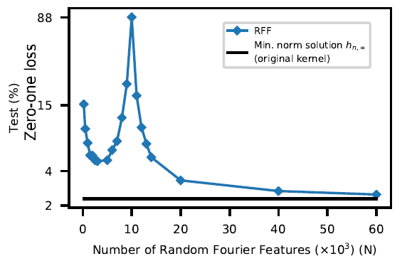
Model-wise double descent risk curve for RFF model on a subset of MNIST (\(n=10^4\), 10 classes), choosing the smallest norm predictor \(h_{n,N}\) when \(N > n\). The interpolation threshold is achieved at \(N=10^4\). Taken from Belkin et al., 2019 ⁴, which uses an equivalent but slightly different definition of RFF models.

Indeed, in the under-parameterized regime, statistical analyses suggest choosing \(N \propto \sqrt{n} \log(n)\) for good test risk guarantees (Rahimi & Recht, 2007). And as we approach the interpolation point (around \(N = n\)), we observe that the test risk increases then decreases again.

In the over-parameterized regime (\(N \geq n\)), multiple predictors are able to fit perfectly the training data. As \(\mathcal{H}_N \in \mathcal{H}_{N+1}\), increasing \(N\) leads to richer model classes and allows constructing interpolating predictors that are more regular, with smaller norm (eventually converging to \(h_{n,\infty}\) obtained from \(\mathcal{H}_{\infty}\)). As detailed in theorem 22 (in a noiseless setting), the small norm inductive bias is indeed powerful to ensure small generalization error.

Theorem 22 (Belkin et al., 2019). Fix any \(h^* \in \mathcal{H}_{\infty}\). Let \((X_1, Y_1), \dots ,(X_n, Y_n)\) be i.i.d. random variables, where \(X_i\) is drawn uniformly at random from a compact cube \(\Omega \in \mathbb{R}^d\), and \(Y_i = h^*(X_i)\) for all \(i\). There exists constants \(A,B > 0\) such that, for any interpolating \(h \in \mathcal{H}_{\infty}\) (i.e., \(h(X_i) = Y_i\) for all \(i\)), so that with high probability :

\[ \sup_{x \in \Omega}|h(x) - h^*(x)| < A e^{-B(n/\log n)^{1/d}} (||h^*||_{\mathcal{H}_{\infty}} + ||h||_{\mathcal{H}_{\infty}}) \]

Proof. We refer the reader directly to Belkin et al., 2019 for the proof. ◻