Deep double descent explained (¼)

15/05/2021

Generalization error: the statistical learning framework and introduction to the phenomenon of double descent

This series of blog posts was co-written with Marc Lafon. Pdf version is available here as well.

\[ \global\def\EMC{\text{EMC}_{P, \epsilon}(\mathcal{T})} \global\def\R{\mathbb{R}} \]

In order to avoid overfitting, conventional wisdom from statistical learning suggests using models that are not too large, or using regularization techniques to control capacity. Yet, in modern deep learning practice, very large over-parameterized models (typically neural networks) are optimized to fit perfectly the training data and still obtain great generalization performance: bigger models are better.

A number of recent articles have observed that, as the model capacity increases, the performance first improves then gets worse (overfitting) until a certain point where it can fit the training data perfectly (interpolation threshold). At this point, increasing model’s capacity actually seems to improve its performance again. This phenomenon, called double descent by Belkin et al., 2019¹, is illustrated in the figure below.

Model-wise double descent: performance after training models without early-stopping. Taken from this blog post

This blog post series (cross-posted here as well) explores the double descent phenomenon as a result of well-chosen inductive biases. This post sets the classical statistical learning framework (following Statistical Learning course by Prof. Gérard Biau) and introduces the phenomenon. By looking at a number of examples, part 2 introduces inductive biases that appear to have a key role in double descent by selecting, among the multiple interpolating solutions, a smooth empirical risk minimizer. Part 3 explores the double descent with two linear models, and part 4 gives other points of view from recent related works.

Generalization error : classical view and modern practice

Definitions and results from statistical learning

In statistical learning theory, the supervised learning problem consists of finding a good predictor \(h_n: \mathbb{R}^d \rightarrow \{0, 1\}\), based on some training data \(D_n\). The data is typically assumed to come from a certain distribution, i.e. \(D_n = \{(X_1, Y_1), \dots, (X_n, Y_n)\}\) is a collection of \(n\) i.i.d. copies of the random variables \((X, Y)\), taking values in \(\mathbb{R}^d \times \{0, 1\}\) and following a data distribution \(P(X, Y)\). We also restrict ourselves to a given class of predictors by choosing \(h_n \in \mathcal{H}\).

Definition 1 (True risk). With \(\ell(h(X), Y) = \mathbb{I}_{(h(X) \neq Y)}\) the 0-1 loss, the true risk (or true error) of a predictor \(h: \mathbb{R}^d \rightarrow \{0, 1\}\) is defined as \[ L(h) = \mathbb{E}[\ell(h(X), Y)] = \mathbb{P}(h(X) \neq Y) \] The true risk is also called the expected risk or the generalization error.

Remark 1. We choose in this section a classification setting, but a regression setting can be adopted as well, for instance with \(Y\) and \(h_n\) taking values in \(\mathbb{R}\) (which we will sometimes do in the subsequent sections). In this case, the 0-1 loss is replaced by other loss functions, such as the squared error loss \(\ell(\hat{y}, y) = (\hat{y} - y)^2\).

In practice, the true distribution of \((X, Y)\) is unknown, so we have to resort to a proxy measure based on the available data.

Definition 2 (Empirical risk). The empirical risk of a predictor \(h: \mathbb{R}^d \rightarrow \mathbb{R}\) on a training set \(D_n\) is defined as:

\[ L_n(h) = \frac{1}{n} \sum_{i=1}^{n} \ell(h(X_i), Y_i) \]

Definition 3 (Bayes risk). A predictor \(h^*: \mathbb{R}^d \rightarrow \{0, 1\}\) minimizing the true risk, i.e. verifying

\[ L(h^*) = \inf_{h: \mathbb{R}^d \rightarrow \{0, 1\}} L(h) \]

is called a Bayes estimator. Its risk \(L^* = L(h^*)\) is called the Bayes risk.

Using \(D_n\), our objective is to find a predictor \(h_n\) as close as possible to \(h^*\).

Definition 4 (Consistency). A predictor \(h_n\) is consistent if

\[ \mathbb{E} L(h_n) \underset{n \rightarrow \infty}{\rightarrow} L^* \]

The empirical risk minimization (ERM) approach ² consists in choosing a predictor that minimizes the empirical risk on \(D_n\) : \(h_n^*\in \text{argmin}_{h \in \mathcal{H}} L_n(h)\). This is something that can be done or approximated in practice, thanks to a wide range of algorithms and optimization procedures, but it is also necessary to ensure that our predictor \(h_n^*\) performs well in general and not only on training data. Depending on the chosen class of predictors \(\mathcal{H}\), statistical learning theory can give us guarantees or insights to make sure \(h_n^*\) generalizes well to unseen data.

Classical view

The gap between any predictor \(h_n \in \mathcal{H}\) and an optimal predictor \(h^*\) can be decomposed as follows. \[ L(h_n) - L^*= \underbrace{L(h_n) - \inf_{h \in \mathcal{H}} L(h)}_{\text{estimation error}} + \underbrace{\inf_{h \in \mathcal{H}} L(h) - L^*}_{\text{approximation error}} \]

Remark 2. In addition to the approximation error (approximating reality with a model) and estimation error (learning a model with finite data) which fits in the statistical learning framework and are the focus of this lecture, there is actually another source of error, the optimization error. This is the gap between the risk of the predictor returned by the optimization procedure (e.g. SGD) and an empirical risk minimizer \(h_n^*\).

Proposition 5. For any empirical risk minimizer \(h_n^* \in \text{argmin}_{h \in \mathcal{H}} L_n(h)\), the estimation error verifies

\[ L(h_n^*) - \inf_{h \in \mathcal{H}} L(h) \leq 2 \sup_{h \in \mathcal{H}} |L_n(h) - L(h)| \]

The term \(|L_n(h) - L(h)|\) is the generalization gap. It is the gap between the empirical risk and the true risk, in other words the difference between a model’s performance on training data and its performance on unseen data drawn from the same distribution.

Proof. We have

\[ L(h_n^*) - \inf_{h \in \mathcal{H}} L(h) \leq |L(h_n^*) - L_n(h_n^*)| + |L_n(h_n^*) - \inf_{h \in \mathcal{H}} L(h)| \]

With

\[ |L(h_n^*) - L_n(h_n^*)| \leq \sup_{h \in \mathcal{H}} |L_n(h) - L(h)| \]

since \(h_n^*\in \mathcal{H}\), and :

\[ |L_n(h_n^*) - \inf_{h \in \mathcal{H}} L(h)| = |\inf_{h \in \mathcal{H}}L_n(h) - \inf_{h \in \mathcal{H}} L(h)| \leq \sup_{h \in \mathcal{H}} |L_n(h) - L(h)| \]

after separating the cases where \(|\inf_{h \in \mathcal{H}}L_n(h) - \inf_{h \in \mathcal{H}} L(h)| > 0\) and \(|\inf_{h \in \mathcal{H}}L_n(h) - \inf_{h \in \mathcal{H}} L(h)| < 0\). ◻

The classical machine learning strategy is to find the right \(\mathcal{H}\) to keep both the approximation error and the estimation error low.

1. When \(\mathcal{H}\) is too small, no predictor \(h \in \mathcal{H}\) is able to model the complexity of the data and to approach the Bayes risk. This is called underfitting.

2. When \(\mathcal{H}\) is too large, the bound from proposition 5 (maximal generalization gap over \(\mathcal{H}\)) will increase, and the chosen empirical risk minimizer \(h_n^*\) may generalize poorly despite having a low training error. This is called overfitting.

Remark 3. Similarly, the expected error can also be decomposed into a bias term due to model mis-specification and a variance term due to random noise being modeled by \(h_n^*\). This is the bias-variance trade-off, and is also highly dependent on the capacity of \(\mathcal{H}\), the chosen class of predictors.

Exercise 1 (Bias-Variance decomposition). Assume that \(Y = h(X) + \epsilon\), with \(\mathbb{E}[\epsilon] = 0, Var(\epsilon) = \sigma^2\). Show that, for any \(x \in \mathbb{R}^d\), the expected error of a predictor \(h_n\) obtained with the random dataset \(D_n\) is :

\[ \mathbb{E}[(Y - h_n(X))^2 | X=x] = (h(x) - \mathbb{E}h_n(x))^2 + \mathbb{E}[(\mathbb{E}h_n(x) - h_n(x))^2] + \sigma^2 \]

In order to ensure a consistent estimator \(h_n\), we can control \(\mathcal{H}\) explicitly e.g. by choosing the number of features used in a linear classifier, or the number of layers of a neural network.

Theorem 6 (Vapnik-Chervonenkis inequality). For any data distribution \(P(X,Y)\), by using \(V_{\mathcal{H}}\) the VC-dimension of the class \(\mathcal{H}\) as a measure of the class complexity, one has

\[ \mathbb{E} \sup_{h\in\mathcal{H}} |L_n(h) - L(h)| \leq 4 \sqrt{\frac{V_{\mathcal{H}} \log(n+1)}{n}} \]

A complete introduction to Vapnik-Chervonenkis theory is outside the scope of this lecture, but VC-dimension \(V_{\mathcal{H}}\) can be defined as the cardinality of the largest set of points that can be shattered, i.e. there is at least one \(h \in \mathcal{H}\) that can assign all possible labels to the set. Combining this result with proposition 5 gives a useful bound on the generalization error for a number of model classes. For instance, if \(\mathcal{H}\) is a class of linear classifiers using \(d\) features (potentially non-linear transformations of input \(x\)), then we have :

\[ V_{\mathcal{H}} \leq d+1 \]

Other measures of the richness of the model class \(\mathcal{H}\) also exist, such as the Rademacher complexity, and can be useful in situations where \(V_{\mathcal{H}} = +\infty\), or in regression settings.

Modern practice

Following results from the first section, a widely adopted view is that, after a certain threshold, “larger models are worse” as they will overfit and generalize poorly. Yet, in modern machine learning practice, very large models with enough parameters to reach almost zero training error are frequently used. Such models are able to fit almost perfectly (i.e. interpolate) the training data and still generalize well, actually performing better than smaller models (e.g. to classify 1.2M examples, AlexNet had 60M parameters and VGG-16 and VGG-19 both exceeded 100M parameters ³). Understanding generalization of overparameterized models in modern deep learning is an active field of research, and we focus on the double descent phenomenon, first demonstrated by Belkin et al., (2019) and illustrated below.

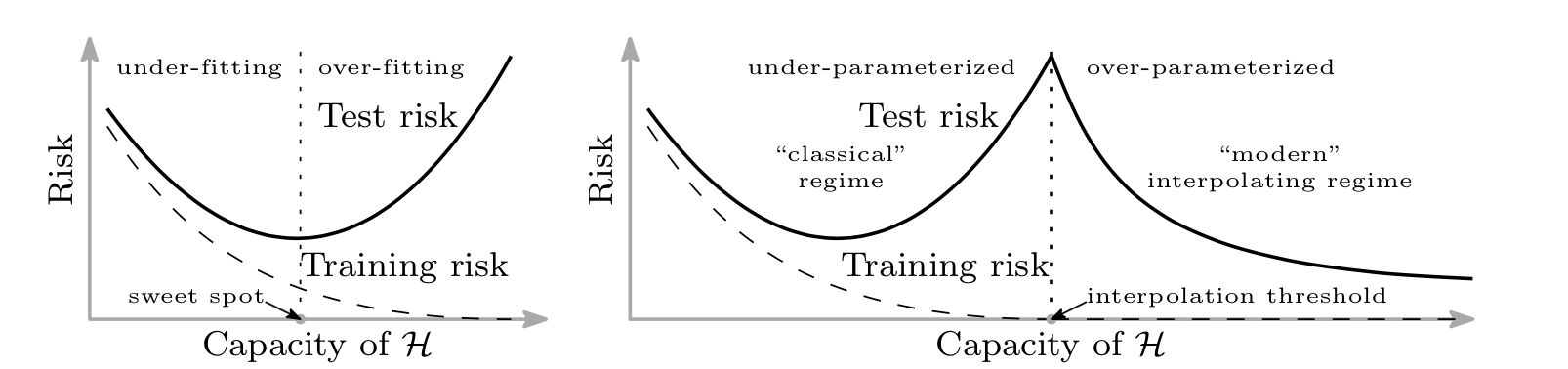
Figure 1. The classical risk curve arising from the bias-variance trade-off and the double descent risk curve with the observed modern interpolation regime. Taken from Belkin et al., (2019).

For simpler class of models, classical statistical learning guarantee that the test risk decreases when the class of models gets more complex, until a point where the bounds do not control the risk anymore. However it seems that, beyond a certain threshold, increasing the capacity of the models actually decreases the test risk again. This is the “modern” interpolating regime, with overparameterized models. As this phenomenon depends not only on the class of predictors \(\mathcal{H}\), but also on the training algorithm and regularization techniques, we define a training procedure \(\mathcal{T}\) to be any procedure that takes as input a dataset \(D_n\) and outputs a classifier \(h_n\), i.e. \(h_n = \mathcal{T}(D_n) \in \mathcal{H}\). We can now make an informal hypothesis, after defining the notion of effective model complexity (from Nakkiran et al. (2019)⁴).

Definition 7 (Effective Model Complexity). The Effective Model Complexity (EMC) of a training procedure \(\mathcal{T}\), w.r.t. distribution \(P(X,Y)\), is the maximum number of samples \(n\) on which \(\mathcal{T}\) achieves on average \(\approx 0\) training error. That is, for \(\epsilon > 0\):

\[ \EMC = \max\{n \in \mathbb{N} | \mathbb{E} L(h_n) \leq \epsilon\} \]

Hypothesis (Generalized Double Descent hypothesis, informal). For any data distribution \(P(X,Y)\), neural-network-based training procedure \(\mathcal{T}\), and small \(\epsilon > 0\), if we consider the task of predicting labels based on \(n\) samples from \(P\) then, as illustrated on figure 1:

• Under-parameterized regime. If \(\EMC\) is sufficiently smaller than n, any perturbation of \(\mathcal{T}\) that increases its effective complexity will decrease the test error.

• Critically parameterized regime. If \(\EMC \approx n\), then a perturbation of \(\mathcal{T}\) that increases its effective complexity might decrease or increase the test error.

• Over-parameterized regime. If \(\EMC\) is sufficiently larger than n, any perturbation of \(\mathcal{T}\) that increases its effective complexity will decrease the test error.

Empirically, this definition of effective model capacity translates into multiple axis along which the double descent can be observed : epoch-wise, model-wise (e.g. increasing the width of convolutional layers or the embedding dimension of transformers) and even with regularization, by decreasing weight decay.

The double descent along different axis of effective model capacity is illustrated in the figures below:

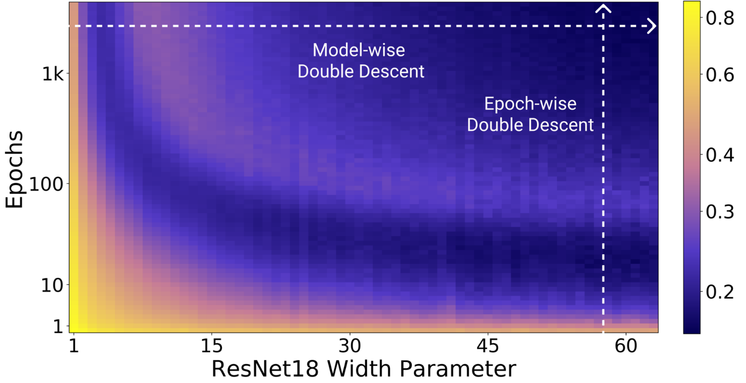
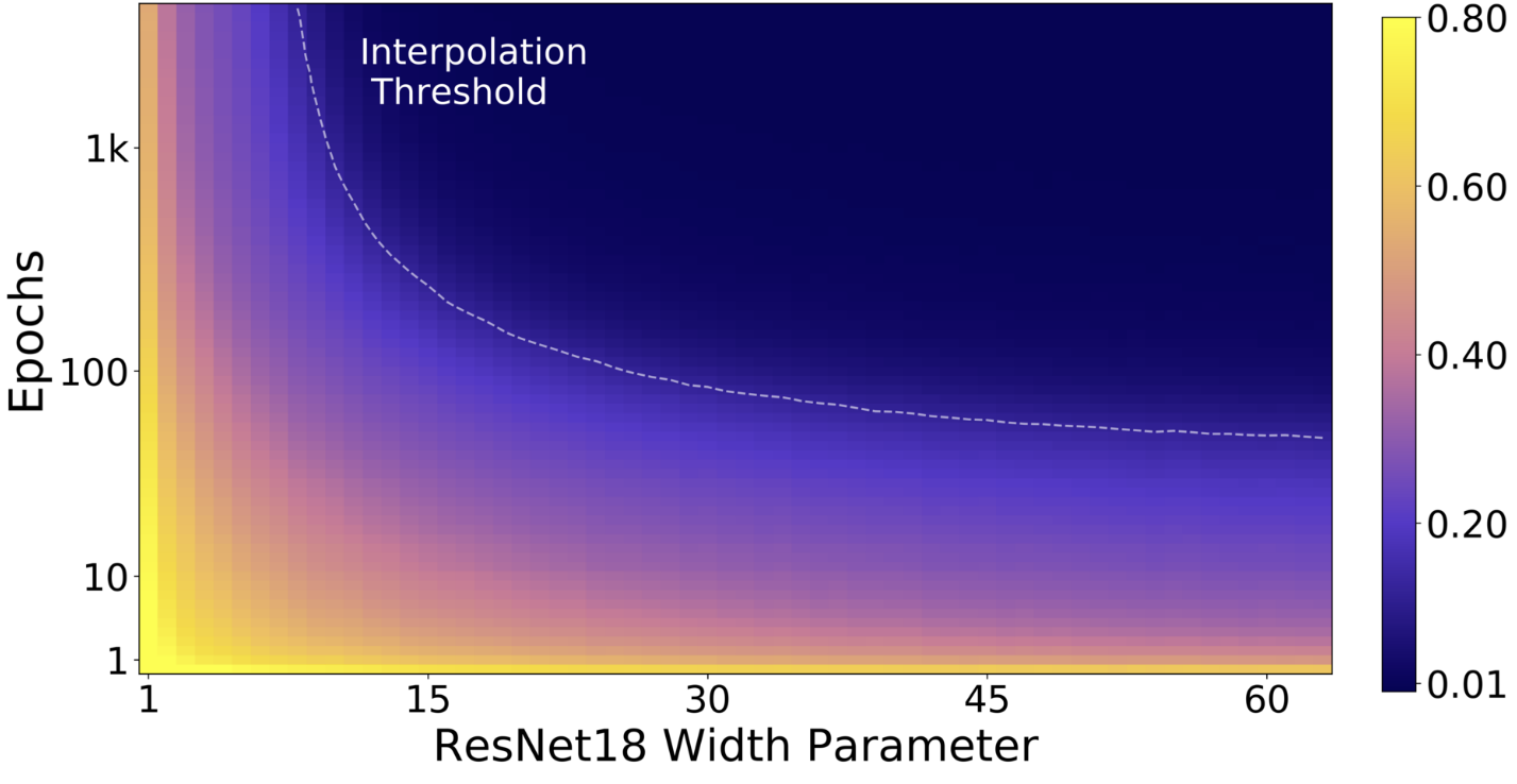
Figure 2. All models are Resnet18s trained on CIFAR-10 with 15% label noise (training labels artificially made incorrect), data-augmentation, and Adam for up to 4K epochs.

Left: test error as a function of model size and train epochs, right: train error of the corresponding models. Taken from Nakkiran et al. (2019).