Variational Auto-Encoder explained

20/08/2021

Reading the original VAE paper (Auto-Encoding Variational Bayes)

\[ \global\def\E{\mathbb{E}} \global\def\R{\mathbb{R}} \]

The Variational Auto-Encoder (VAE) (from Kingma et Welling, 2013 ¹) is an elegant and widely used generative model In contrast with discriminative models which learn the distribution \(p_\theta(y|x)\) (typically classifiers, trained on supervised data to learn a mapping \(f_\theta(x)=y\)), generative models learn the joint distribution \(p_\theta(x,y)\) (or \(p_\theta(x)\) in the case of VAEs). They can be used to generate new data for instance or to do classification using Bayes rule \(p_\theta(y,x)=p_\theta(y|x)p_\theta(x)\), and they typically assume an underlying probabilistic model explaining how the data was generated. in ML, but it relies on several concepts and techniques (variational inference, expectation maximization, etc) which ML/DL practitioners may not be familiar with (at least I wasn’t at the beginning).

Although there are already some well-written blog posts and tutorials on this subject, I thought there would be no harm in clarifying and deriving everything in this post !

The VAE framework and algorithm

Assumptions

The VAE framework relies on a couple assumptions.

First, we assume that the observed data \(x\) follows an underlying distribution

\[x \sim p_{\theta^*}(x|z) \quad \text{for some} \quad z \sim p_{\theta^*}(z)\]

where \(x\) can be images, text², or even graphs³, \(z\) is a latent variable that we cannot observe, and \(\theta^*\) are the optimal parameters of a model that we would like to estimate. This generative process is illustrated in figure below.

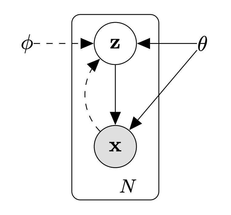
Probabilistic graphical model of the VAE. Solid lines denote the generative model \(p_\theta(z) p_\theta(x|z)\), dashed lines denote the variational approximation \(q_\phi(z|x)\) to the intractable posterior \(p_\theta(z|x)\). Samples are assumed to be i.i.d., with \(N\) the size of our dataset \(\mathcal{D}\), and the latent variables \(z\) are assumed to be local (i.e. one per data point \(x\)), not global. Taken from Kingma et Welling, 2013.

Therefore, our model is made of

• a conditional likelihood \(p_\theta(x \mid z)\) (also called the decoder)
• a prior \(p_\theta(z)\)

This actually defines the following distributions:

• the joint likelihood \(p_\theta(x,z) = p_\theta(x\mid z)p_\theta(z)\)
• the marginal likelihood \(p_\theta(x) = \int_z p_\theta(x,z) dz = \int_z p_\theta(x\mid z)p_\theta(z) dz\)
• the posterior \(p_\theta(z \mid x) = \frac{p_\theta(x,z)}{p_\theta(x)} = \frac{p_\theta(x\mid z)p_\theta(z)}{\int_z p_\theta(x\mid z)p_\theta(z) dz}\)

Since the posterior will typically be intractable analytically (e.g. when \(p_\theta(z \mid x)\) is a neural network), we will approximate it with a model \(q_\phi(z \mid x)\) called the variational posterior, or the encoder.

Since we will be using gradient descent to learn the target distributions \(p_{\theta^*}(x \mid z)\) and \(p_{\theta^*}(z)\), we assume that they come from a parametric family of distributions \(p_\theta(x \mid z)\) and \(p_\theta(z)\), differentiable w.r.t. both \(\theta\) and \(z\).

A common example is to consider a family of Gaussian distributions for the encoder and/or the decoder, with mean and variance specified by a neural network (differentiable w.r.t. its parameters and its inputs). In other words, \(p_\theta(x \mid z) = \mathcal{N}(x; \mu_\theta(z), \sigma_\theta(z))\), where \(\mu_\theta(z)\) and \(\sigma_\theta(z)\) are the outputs of a neural network (MLP, CNN, etc).

Finally, we assume that we are working with continuous latent variables. This will allow us to use the reparametrization trick.

Objectives

As proposed in Kingma et Welling, 2013, VAEs can be used for several purposes, for instance:

• Generative modelling. Once the model is trained, we can use the learned decoder model \(p_\theta(x \mid z)\) to generate artificial data samples, e.g. by sampling from the prior \(p_\theta(z)\) or by interpolating between 2 representations \(z_1 = \mu_z(x_1; \phi)\) and \(z_2 = \mu_z(x_2; \phi)\).
• Representation learning. The encoder \(q_\phi(z \mid x)\) can be used to efficiently approximate \(p_\theta(z \mid x)\), instead of using more expensive sampling methods. This provides a latent representation of the data that is often lower dimension, and can be smoother than a simple auto-encoder model. In the Bayesian vocabulary, computing the posterior probability is called inference, and the VAE allows us to do approximate inference thanks to \(q_\phi(z \mid x)\).
• Authors also mention “efficient approximate marginal inference of the variable \(x\)” (i.e. estimating \(p_\theta(x)\)), but this may be hard when the latent space has a high dimension, and normalizing flows may be a better option

Deriving the variational lower bound (ELBO)

Given a dataset \(\mathcal{D} = (x^{(i)})_{i=1}^N\) and the probabilistic model described above, our objective is to fit our model to the observed data Maximizing the likelihood \(\log p_\theta(x) = \log p(x \mid \theta)\) corresponds to maximum likelihood estimation (MLE), a commonly used estimation framework in ML. But we can also do maximum a posteriori (MAP) estimation in the VAE framework, by choosing a prior \(p(\theta)\) that makes sense, and optimizing instead \(\log p(\theta \mid x) = \log p(x \mid \theta) + \log p(\theta) (-\log p(x))\). Note that this prior \(p(\theta)\) over the parameters is not the same as our prior \(p_\theta(z) = p(z \mid \theta)\) over the latent space. The full derivation with MAP estimation is given in the appendix of Kingma et Welling, 2013.:

\[\max_\theta \log p_\theta(x^{(1)}, \dots, x^{(N)})\]

Since we assumed i.i.d. data, we have

\[\log p(\mathcal{D}) = \log p_\theta(x^{(1)}, \dots, x^{(N)}) = \sum_{i=1}^N \log p_\theta(x^{(i)})\]

And for any \(x\), we have:

\[ \begin{align} \log p_\theta(x) &= \log \frac{p_\theta(x, z)}{p_\theta(z \mid x)} \frac{q_\phi(z \mid x)}{q_\phi(z \mid x)} \tag*{$\forall z, q_\phi$} \\ &= \E_{z \sim q_\phi(z \mid x)} \left[ \log \frac{p_\theta(x, z)}{p_\theta(z \mid x)} \frac{q_\phi(z \mid x)}{q_\phi(z \mid x)} \right] \end{align} \]

test

\[ \begin{align} \log p_\theta(x) &= \log \frac{p_\theta(x, z)}{p_\theta(z \mid x)} \frac{q_\phi(z \mid x)}{q_\phi(z \mid x)} \tag*{$\forall z, q_\phi$} \\ &= \E_{z \sim q_\phi(z \mid x)} \left[ \log \frac{p_\theta(x, z)}{p_\theta(z \mid x)} \frac{q_\phi(z \mid x)}{q_\phi(z \mid x)} \right] \tag*{$\forall q_\phi$} \\ &= \E_{z \sim q_\phi(z \mid x)} \left[ \log \frac{p_\theta(x, z)}{q_\phi(z \mid x)} + \log \frac{q_\phi(z \mid x)}{p_\theta(z \mid x)} \right] \nonumber \\ &= \E_{z \sim q_\phi(z \mid x)} \left[ \log \frac{p_\theta(x, z)}{q_\phi(z \mid x)} \right] + D_{KL} [q_\phi(z \mid x) \mid \mid p_\theta(z \mid x) ] \end{align} \]

We know how to compute \(p_\theta(x, z) = p_\theta(x \mid z) p_\theta(z)\) and \(q_\phi(z \mid x)\), but not the true posterior \(p_\theta(z \mid x)\). Since the KL divergence between two distributions is always positive, we can actually maximize \(\log p_\theta(x)\) by simply maximizing the left term:

\[\begin{align} \mathcal{L}_{ELBO}(\theta, \phi; x) &= \E_{z \sim q_\phi(z \mid x)} \left[ \log \frac{p_\theta(x, z)}{q_\phi(z \mid x)} \right] \nonumber \\ &= \E_{z \sim q_\phi(z \mid x)} \left[ \log p_\theta(x \mid z) + \log \frac{p_\theta(z)}{q_\phi(z \mid x)} \right] \\ &= \E_{z \sim q_\phi(z \mid x)} [\log p_\theta(x \mid z)] - D_{KL} [p_\theta(z) \mid \mid q_\phi(z \mid x)] \end{align}\]

Since we have \(\log p_\theta(x) \geq \mathcal{L}_{ELBO}(\theta, \phi; x)\) and we are using a variational distribution \(q_\phi(z \mid x)\) (i.e. simply an approximation of the true posterior), this term is called the variational lower bound. It is also known as the Evidence lower bound, or ELBO.

Deriving the actual training objective and algorithm

Optimizing the ELBO instead of the likelihood \(p_\theta(x)\) is not specific to the VAE, and is often done in Bayesian inference (e.g. the EM algorithm, or Variational Bayes). Next section provides additional details, and justification of why this works.

In the VAE framework however, thanks to our assumptions on \(p_\theta\) and \(q_\phi\) (they are differentiable w.r.t. \(\theta\), \(\phi\) and \(z\), and they allow the reparameterization trick), we can optimize the ELBO objective simply by gradient ascent ! This allows us to train the model like a regular deep learning model, with mini-batch updates on large datasets, using large and expressive models if we want to.

Computing the gradient w.r.t. \(\theta\)

The gradient of the ELBO objective w.r.t. \(\theta\) can be estimated with a simple Monte-Carlo estimate, since the expectation does not depend on \(\theta\): \[ \begin{align*} \nabla_\theta \mathcal{L}_{ELBO}(\theta, \phi; x) &= \nabla_\theta \E_{z \sim q_\phi(z \mid x)} \left[ \log \frac{p_\theta(x, z)}{q_\phi(z \mid x)} \right] \\ &= \E_{z \sim q_\phi(z \mid x)} \left[\nabla_\theta \log \frac{p_\theta(x \mid z) p_\theta(z)}{q_\phi(z \mid x)} \right] \\ &\approx \frac{1}{L} \sum_{l=1}^L \left[\nabla_\theta \log \frac{p_\theta(x \mid z^{(l)}) p_\theta(z^{(l)})}{q_\phi(z^{(l)} \mid x)} \right] \tag*{with $z^{(l)} \sim q_\phi(z \mid x)$} \end{align*} \]

Or, if using eq. \((3)\):

\[\nabla_\theta \mathcal{L}_{ELBO}(\theta, \phi; x) \approx - \nabla_\theta D_{KL} [p_\theta(z) \mid \mid q_\phi(z \mid x)] + \frac{1}{L} \sum_{l=1}^L \left[\nabla_\theta \log p_\theta(x \mid z^{(l)})\right]\]

Computing the gradient w.r.t. \(\phi\) (the reparametrization trick)

However for \(\phi\), this is more complex since we cannot simply “push” the gradient inside the expectation. Or is it? For many distributions Section 2.4 of the VAE paper gives more details, but this includes several common distributions, notably Gaussian, Exponential, Laplace, etc, and some compositions of these distributions., we can actually use the reparametrization trick by re-writing our sampling process:

\[z \sim q_\phi(z \mid x) \Leftrightarrow \begin{cases} \epsilon \sim p(\epsilon) \\ z = g_\phi(\epsilon, x) \end{cases}\]

with \(g_\phi\) a differentiable function.

For instance, if we consider Gaussian distributions for our encoder, i.e. \(q_\phi(z \mid x) = \mathcal{N}(z; \mu_\phi(x), \sigma_\phi(x))\), we can simply sample \(\epsilon \sim \mathcal{N}(0,1)\) and obtain \(z = g_\phi(\epsilon, x) = \mu_\phi(x) + \epsilon \sigma_\phi(x)\).

This allows to compute a practical estimator of the ELBO gradient w.r.t. \(\phi\) as well.

For any function \(f\), we have:

\[\begin{align*} \nabla_\phi \E_{z \sim q_\phi(z \mid x)} [f(z)] &= \nabla_\phi \E_{\epsilon \sim p(\epsilon)} [f(g_\phi(\epsilon, x))] \\ &= \E_{\epsilon \sim p(\epsilon)} \nabla_\phi [f(g_\phi(\epsilon, x))] \\ &\approx \frac{1}{L} \sum_{l=1}^L \nabla_\phi [f(g_\phi(\epsilon^{(l)}, x))] \end{align*}\]

which can be computed if \(f\) and \(g_\phi\) are differentiable w.r.t. \(z\) and \(\phi\) respectively.

Therefore, by using the reparametrization trick, we can simply compute the following estimators and back-propagate w.r.t. \(\phi\) (using respectively eq. \((2)\) and \((3)\)):

\[\nabla_\phi \mathcal{L}_{ELBO}(\theta, \phi; x) \approx \frac{1}{L} \sum_{l=1}^L \nabla_\phi \left( \log p_\theta(x, z^{(l)}) - \log q_\phi(z^{(l)} \mid x) \right)\]

or

\[\nabla_\phi \mathcal{L}_{ELBO}(\theta, \phi; x) \approx - \nabla_\phi D_{KL} [p_\theta(z) \mid \mid q_\phi(z \mid x)] + \frac{1}{L} \sum_{l=1}^L \nabla_\phi \log p_\theta(x \mid z^{(l)})\]

with \(\epsilon^{(l)} \sim p(\epsilon)\) a sample and \(z^{(l)} = g_\phi(\epsilon^{(l)}, x)\) now a differentiable function of \(\phi\). This is the step that requires \(z\) to be continuous, and makes it hard to work with discrete latent variables (e.g. text)One solution to use discrete latent variables in the VAE framework is to use the Gumbel-softmax trick, see ⁴.

In practice, thanks to auto-diff in modern DL frameworks (PyTorch, Tensorflow), it is enough to sample \(z^{(l)}\) with the reparametrization trick (\(z^{(l)} = g_\phi(\epsilon^{(l)}, x)\)), compute the ELBO loss:

\[\mathcal{\widetilde{L}}^A_{ELBO}(\theta, \phi; x) = \frac{1}{L} \sum_{l=1}^L \log p_\theta(x, z^{(l)}) - \log q_\phi(z^{(l)} \mid x)\]

or

\[\mathcal{\widetilde{L}}^B_{ELBO}(\theta, \phi; x) = - D_{KL} [p_\theta(z) \mid \mid q_\phi(z \mid x)] + \frac{1}{L} \sum_{l=1}^L \log p_\theta(x \mid z^{(l)})\]

and obtain the gradients w.r.t. both \(\phi\) and \(\theta\) by simply calling elbo_loss.backward(). Authors call \(\mathcal{\widetilde{L}}_{ELBO}(\theta, \phi; x)\) the Stochastic Gradient Variational Bayes estimator.

Note: another option to estimate this gradient is to use the log-trick (\(\nabla f = f \nabla \log f\)) to obtain the following:

\[\begin{align*} \nabla_\phi \E_{z \sim q_\phi(z \mid x)} [f(z)] &= \E_{z \sim q_\phi(z \mid x)} [f(z) \nabla_\phi \log q_\phi(z \mid x)] \\ &\approx \frac{1}{L} \sum_{l=1}^L f(z^{(l)}) \nabla_\phi \log q_\phi(z^{(l)} \mid x) \end{align*}\]

Therefore

\[\begin{align*} \nabla_\phi \mathcal{L}_{ELBO}(\theta, \phi; x) &\approx - \nabla_\phi D_{KL} [p_\theta(z) \mid \mid q_\phi(z \mid x)] \\ &+ \frac{1}{L} \sum_{l=1}^L \log p_\theta(x \mid z^{(l)}) \nabla_\phi \log q_\phi(z^{(l)} \mid x) \end{align*}\]

with \(z^{(l)} \sim q_\phi(z \mid x)\) sampled directly, and not a function of \(\phi\) anymore.

This allows discrete latent variables since it does not require differentiating through \(z\), however this estimator suffers from a high variance ⁵.

The algorithm

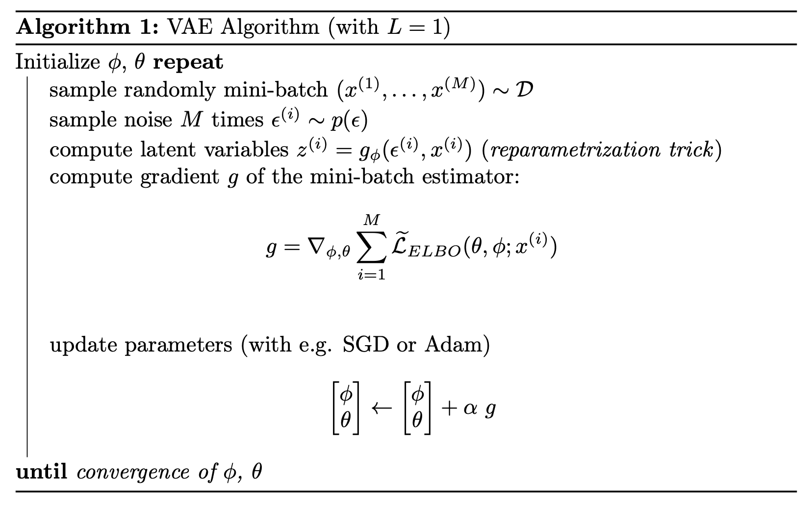
In order to work with large datasets, we can do mini-batch optimization and use only \(M\) samples of \(\mathcal{D}\) at each training step. With \(M\) large enough, we do not need many latent variable samples, and we can actually use \(L=1\).

Here is finally the VAE algorithm (initially called Auto-Encoding Variational Bayes or AEVB algorithm by the authors):

The link with EM and Variational Bayes

Optimizing the ELBO over model parameters \(\theta\) and a distribution \(q\), in order to maximize the likelihood on the dataset, is not unique to the VAE framework. Remember eq. \((1)\):

\[\log p_\theta(x) = \mathcal{L}_{ELBO}(\theta, q; x) + D_{KL}[q(z \mid x) \mid \mid p_\theta(z \mid x)] \tag*{$\forall q$}\]

The gap between the marginal likelihood \(p_\theta(x)\) and our ELBO is illustrated in the figure below:

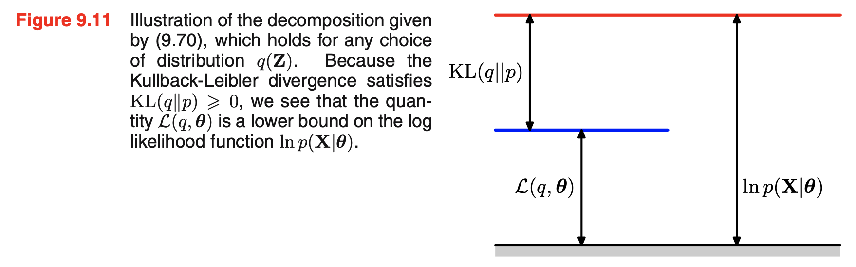
Taken from Bishop, 2006, chapter 9.4.

The Expectation Maximization algorithm

The EM algorithm can be used when we are able to compute the exact posterior \(p_\theta(z \mid x)\), for any \(\theta\). We can then alternate between the 2 following steps, iteratively until convergence:

• E step. Compute \(q_t(z \mid x) = p_{\theta_t}(z \mid x)\). This brings the gap between the ELBO and the log likelihood down to zero.
• M step. While keeping the variational distribution \(q_t\) fixed, maximize \(\mathcal{L}_{ELBO}(\theta, q_t)\) w.r.t. \(\theta\) to obtain new parameters \(\theta_{t+1}\). This will improve the ELBO term of eq. \((1)\) but will also increase the KL divergence term, therefore it will necessarily improve the log likelihood \(\log p_\theta(x)\).

Example: Mixtures of Gaussians. (taken from Bishop, Pattern Recognition and Machine Learning Bishop, 2006, chapter 9.2 ⁶)

---

Let’s consider that our data \(x \in \R^d\) comes from a mixture of \(K\) Gaussian distributions with means \(\mu_k \in \R^d\) and covariance matrices \(\Sigma_k \in \R^{d\times d}\):

\[p(x)= \sum_{k=1}^K \pi_k \mathcal{N}(x \mid \mu_k, \sigma_k)\]

with \(\pi_k \in [0,1] \ \forall k\) the mixture coefficients, such that \(\sum_k \pi_k = 1\). By introducing the latent vector \(z \in \{0,1\}^K\), following the categorical distribution defined by coefficients \(\pi_k\) and one-hot encoded (i.e. \(\exists! k \in [1,K], z_k = 1\)), we have:

\[\begin{align*} &\forall k, p(z_k = 1) = \pi_k \\ &\forall z \in p(z) = \prod_{k=1}^K \pi_k^{z_k} \\ &\forall x, p(x) = \sum_z p(z) p(x \mid z) \end{align*}\]

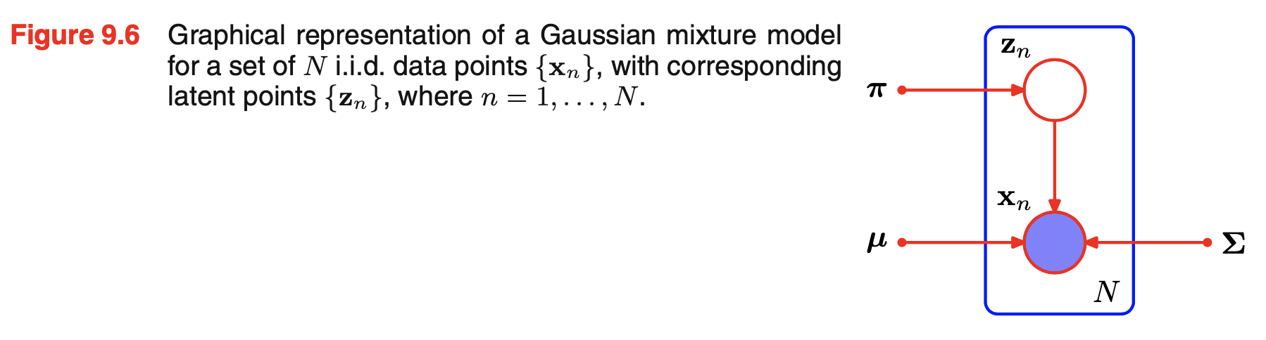
This probabilistic model is represented in figure below, with \(x_n\) our datapoints, \(z_n\) the underlying latent variable (that can be seen as “which of the Gaussian distributions are we sampling from”) and \(\theta = (\pi_k, \mu_k, \Sigma_k)_{k\in[1,K]}\) our model parameters to optimize.

Taken from Bishop, 2006, chapter 9.2.

Deriving the equations is a good exercise (done in the book), but with this model, we can compute everything analytically to apply the EM algorithm.

• E step. The true posterior \(p_\theta(z \mid x) = p(z \mid x, \pi, \mu, \Sigma)\) is obtained:

\[\forall k, p(z_k = 1 \mid x) =\frac{\pi_{k} \mathcal{N}\left(x \mid \mu_{k}, \Sigma_{k}\right)}{\sum_{j=1}^{K} \pi_{j} \mathcal{N}\left(x \mid \mu_{j}, \Sigma_{j}\right)}\]

• M step. With our variational distribution set to the true posterior, our ELBO actually becomes equal to the marginal likelihood \(p(x)\), that we can express and differentiate analytically w.r.t. its parameters (in this particular case of the Gaussian mixture model). By taking the derivative or using a Lagrange multiplier (for \(\pi_k\), constrained to the simplex), we obtain estimates of the optimal parameters:

\[\begin{aligned} \mu_{k}^{\text{new}} &=\frac{1}{N_{k}} \sum_{n=1}^{N} \gamma\left(z_{n k}\right) x_{n} \\ \Sigma_{k}^{\text{new}} &=\frac{1}{N_{k}} \sum_{n=1}^{N} \gamma\left(z_{n k}\right) \left(x_{n}-\mu_{k}^{\text{new}}\right) \left(x_{n}-\mu_{k}^{\text{new}}\right)^T \\ \pi_{k}^{\text{new}} &=\frac{N_{k}}{N} \end{aligned}\]

with \(N_k = \sum_{n=1}^N \gamma(z_{nk})\) and \(\gamma(z_{nk}) = p(z_{nk} = 1 \mid x_n)\) our updated updated values for the posterior.

In this case, the EM algorithm consists in alternating between these 2 steps until a convergence criterion is met (on the parameters or the log likelihood).

---

In the case where either the M-step or the E-step is instractable, and analytic solutions cannot be found, the generalized EM algorithm consists in simply increasing the value of the ELBO \(\mathcal{L}_{ELBO}(\theta, q)\) iteratively, instead of fully maximizing it w.r.t. \(q\) (E-step) and then \(\theta\) (M-step), multiple times.

This is enough to maximize the log likelihood, since any global maximum \(q^*, \theta^*\) of \(\mathcal{L}_{ELBO}\) will be a global maximum of \(\log p_\theta(x)\). Indeed, the optimal \(q^*\) is always determined by \(\theta\) and equals the true posterior \(p_\theta(z \mid x)\). Therefore, any maximum \(q^*, \theta^*\) of the ELBO is also a maximum of \(\log p_\theta(x)\) (otherwise it would mean that we could find another \(\theta\) increasing both the log likelihood and the ELBO).

Variational Bayes

Variational Bayes, also known as variational inference or approximate inference encompasses various methods (including VAEs) to do inference and/or learn probabilistic models, when the posterior \(p_\theta(z \mid x)\) is instractable.

The main idea behind is to restrict our optimization problem \(\max_{q, \theta} \mathcal{L}_{ELBO}(\theta, q)\) to a class of tractable distributions \(q \in \mathcal{Q}\), instead of searching over all possible distributions. This means that we may not be able to match the true posterior, but given a well-suited or large enough class \(Q\), we can approximate it This implies that, the larger our class \(Q\) of encoders, the better we may approximate the true posterior. This approximation is imposed only for tractability, and will not lead to overfitting. This is not true regarding the model \(p_\theta(x \mid z)\) (VAE decoder), where more flexible functions can lead to issues such as KL vanishing..

Among the multiple variational inference methods, proposing different way to parametrize \(\mathcal{Q}\) (e.g. distributions of the exponential family with simple parameters, Gaussian processes, neural networks based distributions, etc), a classical and very well known method is called mean-field inference ⁷. It relies on the assumption that we can factorize our variational distribution

\[q(z) = \prod_{i=1}^M q(z_i)\]

where \(z = (z_1, \dots z_M)\) can be any separation we want, e.g. on the coordinates (reducing our distribution on a vector \(z\in \R^M\) to a product of distributions over scalars). This allows to compute the ELBO

\[\mathcal{L}_{ELBO}(\theta, \phi; x) = \E_{z \sim q_\phi(z \mid x)} \left[ \log \frac{p_\theta(x, z)}{q_\phi(z \mid x)} \right]\]

analytically, and derive an optimization procedure. More details and examples can be found in Bishop’s book, chapter 10.

The VAE algorithm (initially called Autoencoding Variational Bayes) is a variational inference method as well, but:

• it does not require computing the expectation over \(q_\phi(z \mid x)\) analytically, therefore we have more freedom on the choice of the class of variational distributions. Compared to mean-field for instance, we can choose large and complex neural networks to parametrize \(q_\phi(z \mid x)\).
• the optimization procedure with mini-batch gradient descent does allow to work with large datasets.

Note: In addition to variational inference methods, sampling-based methods have also been developped to work with intractable posteriors (e.g. MCMC methods: Gibbs sampling, Metropolis-Hastings). Contrarily to variational methods which restrict the optimization to a class of distributions, they don’t make this assumption and are guaranteed to find a global optimum given enough time. In practice however, they can be computationally very expensive. More details in this blog post.

Additional notes

The Wake-Sleep algorithm ⁸ is mentioned as an alternative method to do variational inference that scales well to large datasets and deep networks. Like the EM algorithm, it alternates between 2 phases (“wake” phase = M-step, “sleep” phase = E-step). Like the VAE algorithm, it learns an approximation of the true posterior (our variational posterior, \(q_\phi(z \mid x)\)), but unlike the VAE, it can be applied to models with discrete latent variables (see e.g. ⁹)). However, it does not optimize (a bound) of the marginal likelihood, and is therefore biased. There has been some work showing the connections between the Wake Sleep algorithm, VAEs and even GANs (see ¹⁰).

In this post, we introduced and explained the VAE algorithm through the lens of variational inference, deriving the training objective (ELBO loss) from the model likelihood on the data \(\log p_\theta(\mathcal{D})\). But the resulting model is actually close to other well-known models in ML/DL, in the auto-encoders family. Compared to the vanilla auto-encoder model, it can be seen as a probabilistic extension with the added KL divergence term acting as a regularizer, to ensure a smooth latent space. This blog post summarizes nicely the various models in the auto-encoder family (including the \(\beta\)-VAE or Beta-VAE, an extension that can help alleviate the KL vanishing issue).